Stringing Stress Calculation Methods | Articles

Transmission tower with digital data overlay

Abstract

The article compares methods for calculating stringing stresses in overhead line conductors while accounting for permanent deformation. Two approaches are considered: a nonlinear method based on conductor elongation curves, and a linear method using coefficients for initial elongation and after creep elongation. A comparative calculation for ACSR 500/64 shows a difference of no more than 5%. An algorithm for comparative calculation is developed for cases where the experimental data required by both methods are available, and the need for further development of the regulatory and technical framework is noted.

UDC 621.3

1. Background and Calculation Approaches

In the second half of the twentieth century, methods for accounting for permanent conductor deformation based on experimental data were developed almost simultaneously in the United States [1] and the Soviet Union [2, 3]. As a result, two principal approaches to accounting for conductor elongation on overhead lines emerged.

The first approach, widely adopted in Western countries, determines elongation from nonlinear conductor elongation curves. In the Soviet Union, the Central Asian division of Energosetproekt developed temporary guidelines [4], in which permanent deformation was described using linear coefficients for initial elongation and after creep elongation. The guidelines were explicitly temporary, intended for 2-3 years, and required subsequent refinement based on additional research and operating experience. Nevertheless, the method continues to be used in Russia because no alternative regulatory approach has been established that combines a unified test methodology with broad adoption by test laboratories and domestic software developers.

Both approaches depend on expensive experimental testing. Determination of conductor characteristics requires long-duration tensile testing under constant load: at least 1,000 hours at each load step under [5], and 10-30 days under [4]. In Western practice, where the conductor catalogue exceeds 5,000 types [6], such test data are not always available at the design stage. Simplified approaches may therefore be used, including a linear elongation-stress assumption with a temperature shift between initial elongation and after creep elongation curves [1].

Three principal approaches can therefore be identified: linear coefficients for initial elongation and after creep elongation; nonlinear coefficients for initial elongation and after creep elongation, described in detail in [7]; and a temperature shift between initial elongation and after creep elongation curves represented by linear relationships. The third method is the least preferable because the shift is inferred from conductor characteristics rather than directly established by testing. The comparison below therefore focuses on the first two methods.

2. Example Conductor and Input Data

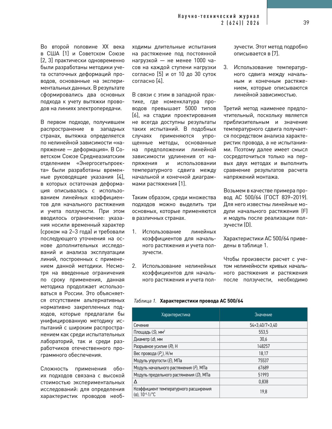
The example conductor is ACSR 500/64 manufactured to GOST 839-2019. For this conductor, the linear initial elongation modulus F and the after creep elongation modulus D are known.

Table 1. Example conductor characteristics
Characteristic	Value
Stranding	54 x 3.40 / 7 x 3.40
Cross-sectional area S, mm²	553.5
Diameter d, mm	30.6
Rated breaking strength R, N	148,257
Conductor weight \(P_p\), N/m	18.17
Modulus of elasticity E, MPa	75,537
Initial elongation modulus F, MPa	67,689
After creep elongation modulus D, MPa	51,993
Δ	0.838
Coefficient of thermal expansion α, 10^-6/°C	19.8

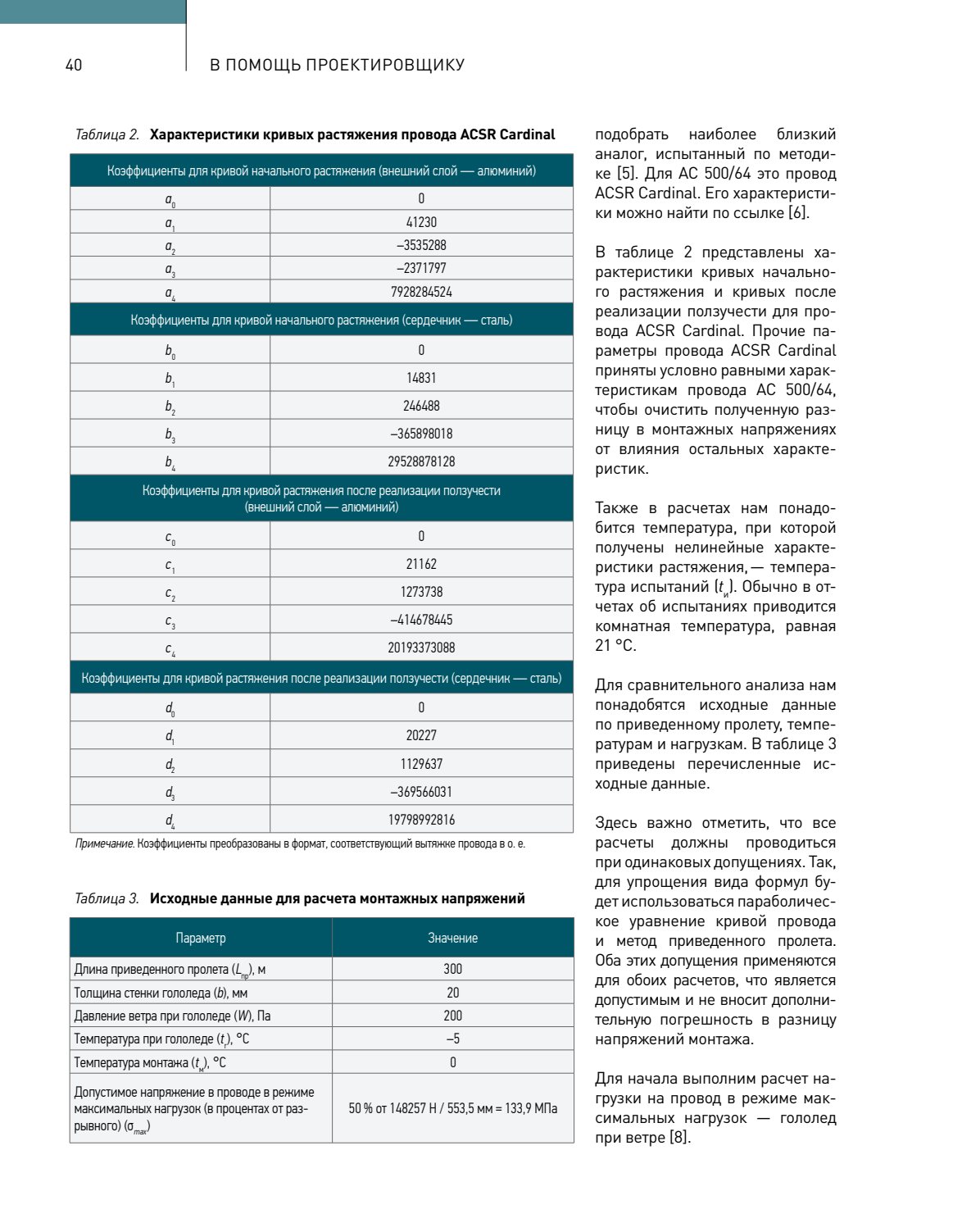
To perform the nonlinear calculation, the closest comparable conductor tested in accordance with [5] is selected. For ACSR 500/64 this is ACSR Cardinal. Other ACSR Cardinal parameters are assumed to be equal to those of ACSR 500/64 so that the difference in stringing stress reflects only the elongation model rather than other conductor characteristics.

Table 2. Elongation curve coefficients for ACSR Cardinal
Elongation curve / component	0	1	2	3	4
Initial elongation - aluminium, a	a₀ = 0	a₁ = 41,230	a₂ = -3,535,288	a₃ = -2,371,797	a₄ = 7,928,284,524
Initial elongation - steel core, b	b₀ = 0	b₁ = 14,831	b₂ = 246,488	b₃ = -365,898,018	b₄ = 29,528,878,128
After creep elongation - aluminium, c	c₀ = 0	c₁ = 21,162	c₂ = 1,273,738	c₃ = -414,678,445	c₄ = 20,193,373,088
After creep elongation - steel core, d	d₀ = 0	d₁ = 20,227	d₂ = 1,129,637	d₃ = -369,566,031	d₄ = 19,798,992,816

Note: the coefficients are converted to a format corresponding to conductor strain expressed in per-unit values. The nonlinear test temperature is taken as 21°C, a typical room temperature reported in conductor test data.

Table 3. Input data for stringing stress calculation
Parameter	Value
Ruling span \(L_{eq}\), m	300
Radial ice thickness b, mm	20
Wind pressure under icing \(W\), Pa	200
Icing temperature \(t_g\), °C	-5
Stringing temperature \(t_m\), °C	0
Allowable stress under maximum load \(\sigma_{max}\)	50% of 148,257 N / 553.5 mm² = 133.9 MPa

All comparative calculations must use the same assumptions. A parabolic conductor equation and the ruling-span method are therefore used in both calculations. Because the assumptions are identical, they do not introduce additional error into the difference between the calculated stringing stresses.

3. Maximum Conductor Loading

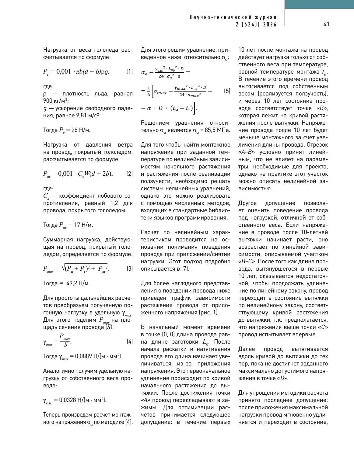
The maximum-load case is taken as ice combined with wind [8]. The ice weight per unit length is calculated from:

P_g = 0.001 \cdot \pi \cdot b(d+b) \cdot \rho \cdot g \tag{1}

where \(\rho = 900\ \mathrm{kg/m^3}\) is ice density and \(g = 9.81\ \mathrm{m/s^2}\) is gravitational acceleration. This gives \(P_g = 28\ \mathrm{N/m}\).

The wind load on the ice-covered conductor is:

P_{Wg} = 0.001 \cdot C_x \cdot W(d+2b) \tag{2}

where \(C_x = 1.2\) is the drag coefficient for an ice-covered conductor. This gives \(P_{Wg} = 17\ \mathrm{N/m}\).

The resultant maximum load is:

P_{max} = \sqrt{(P_p + P_g)^2 + P_{Wg}^2} = 49.2\ \mathrm{N/m} \tag{3}

\gamma_{max} = \frac{P_{max}}{S} = 0.0889\ \mathrm{N/(m \cdot mm^2)} \tag{4}

Analogously, the unit load due to conductor self-weight is:

\gamma_{SW} = 0.0328\ \mathrm{N/(m \cdot mm^2)}

4. Linear-Method Stringing Stress

The stringing stress \(\sigma_m\) is first calculated in accordance with method [4]. The conductor state equation is solved for \(\sigma_m\) using the maximum-load and self-weight conditions, temperature difference, ruling span and after creep elongation modulus D:

\sigma_m - \frac{\gamma_{SW}^{2} L_{eq}^{2} D} {24 \sigma_m^{2} \Delta} = \frac{1}{\Delta} \left[ \sigma_{max} - \frac{\gamma_{max}^{2} L_{eq}^{2} D} {24 \sigma_{max}^{2}} - \alpha D(t_m - t_g) \right] \tag{5}

The solution is \(\sigma_m = 85.5\ \mathrm{MPa}\).

5. Nonlinear Elongation Method

Determining stringing stress at a specified temperature from nonlinear initial elongation and after creep elongation relationships requires the solution of systems of nonlinear equations. This can be implemented using numerical methods available in standard programming-language libraries. The calculation is based on the conductor response during loading and unloading, as described in [7].

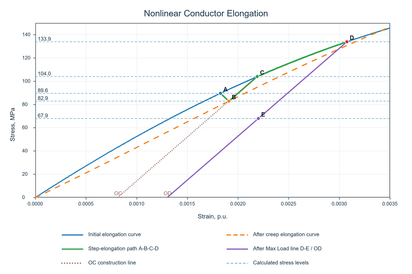
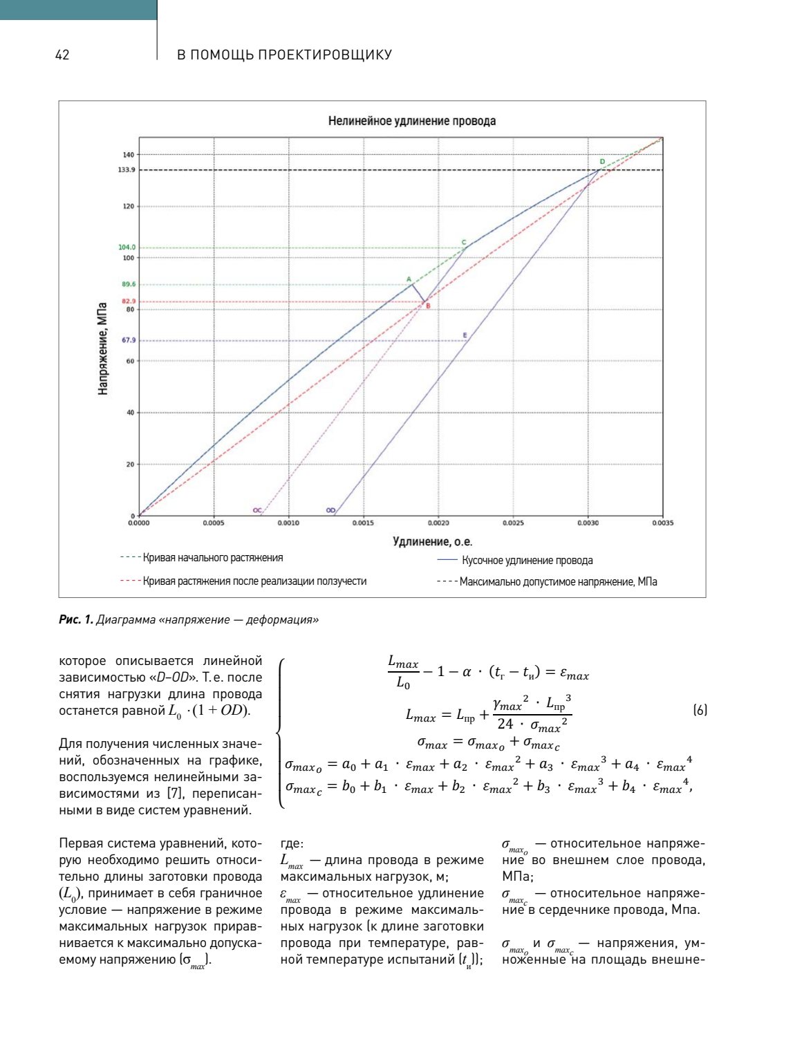
Figure 1. Nonlinear conductor elongation diagram.

At the initial point (0, 0), the conductor length is equal to the manufactured length \(L_0\). During paying out and tensioning, the conductor elongates along the initial elongation curve until point A is reached. The conductor is then clipped in. For the calculation, it is assumed that during the first 10 years after installation the conductor is subjected only to self-weight at the stringing temperature \(t_m\). Creep develops and the conductor moves to point B on the after creep elongation curve. The stress after 10 years is lower than the original stringing stress because the conductor has elongated.

The A-B segment of the step-elongation path is treated as linear. If stress then increases above the 10-year condition, the response follows the linear B-C segment. Once this linear extension is exhausted, the conductor returns to the nonlinear initial elongation curve because stresses above point C are assumed to be experienced for the first time. The conductor continues along that curve to the maximum allowable stress at point D. Finally, after the maximum load is removed, an immediate permanent extension is assumed and the conductor follows the unloading line D-OD; the unloaded length therefore remains \(L_0(1 + OD)\).

6. Determination of Original Conductor Length

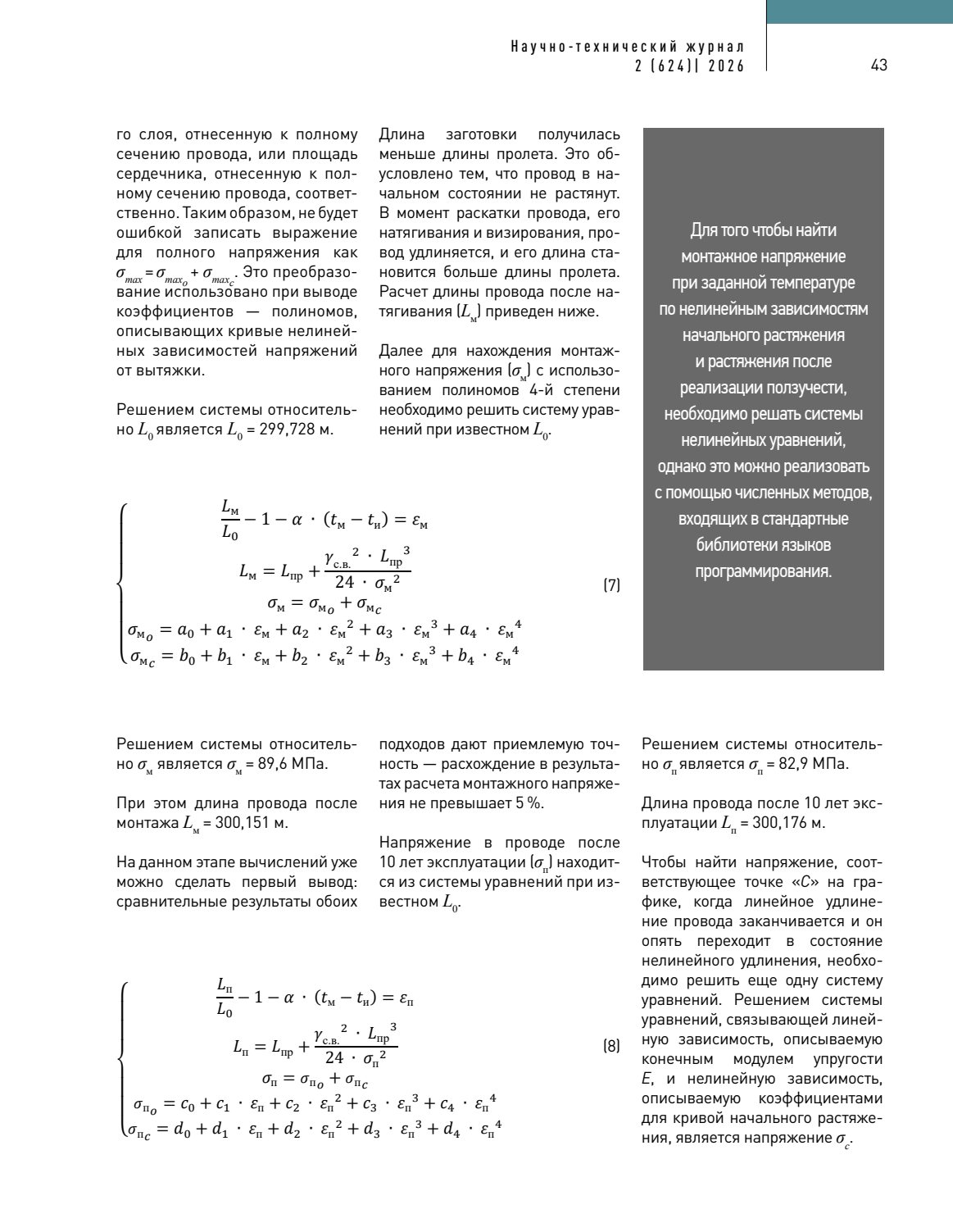
The first nonlinear system is solved for the original conductor length \(L_0\). The boundary condition is that stress under the maximum-load condition equals the allowable maximum stress \(\sigma_{max}\). The fourth-order polynomial expressions separately represent the outer aluminium layer and steel core, and their contributions are summed to obtain the total conductor stress.

\left\{ \begin{array}{l} \frac{L_{max}}{L_0} - 1 - \alpha(t_g - t_i) = \varepsilon_{max} \\ L_{max} = L_{eq} + \frac{\gamma_{max}^{2} L_{eq}^{3}}{24 \sigma_{max}^{2}} \\ \sigma_{max} = \sigma_{max,o} + \sigma_{max,c} \\ \sigma_{max,o} = a_0 + a_1\varepsilon_{max} + a_2\varepsilon_{max}^{2} + a_3\varepsilon_{max}^{3} + a_4\varepsilon_{max}^{4} \\ \sigma_{max,c} = b_0 + b_1\varepsilon_{max} + b_2\varepsilon_{max}^{2} + b_3\varepsilon_{max}^{3} + b_4\varepsilon_{max}^{4} \end{array} \right. \tag{6}

Here \(t_i\) is the nonlinear test temperature. The solution is \(L_0 = 299.728\ \mathrm{m}\). The original conductor length is shorter than the span because the conductor is initially unstressed; during paying out, tensioning and sagging it elongates and its actual length becomes greater than the span length.

7. Nonlinear Stringing Stress and 10-Year Condition

With \(L_0\) known, the stringing stress is obtained by solving the fourth-order polynomial system for the stringing condition:

\left\{ \begin{array}{l} \frac{L_m}{L_0} - 1 - \alpha(t_m - t_i) = \varepsilon_m \\ L_m = L_{eq} + \frac{\gamma_{SW}^{2} L_{eq}^{3}}{24 \sigma_m^{2}} \\ \sigma_m = \sigma_{m,o} + \sigma_{m,c} \\ \sigma_{m,o} = a_0 + a_1\varepsilon_m + a_2\varepsilon_m^{2} + a_3\varepsilon_m^{3} + a_4\varepsilon_m^{4} \\ \sigma_{m,c} = b_0 + b_1\varepsilon_m + b_2\varepsilon_m^{2} + b_3\varepsilon_m^{3} + b_4\varepsilon_m^{4} \end{array} \right. \tag{7}

The solution is \(\sigma_m = 89.6\ \mathrm{MPa}\), with a conductor length after stringing of \(L_m = 300.151\ \mathrm{m}\). The comparison already shows acceptable agreement between the two methods: the difference in calculated stringing stress is less than 5%.

The conductor stress after 10 years of operation is then found from the after creep elongation polynomial system:

\left\{ \begin{array}{l} \frac{L_p}{L_0} - 1 - \alpha(t_m - t_i) = \varepsilon_p \\ L_p = L_{eq} + \frac{\gamma_{SW}^{2} L_{eq}^{3}}{24 \sigma_p^{2}} \\ \sigma_p = \sigma_{p,o} + \sigma_{p,c} \\ \sigma_{p,o} = c_0 + c_1\varepsilon_p + c_2\varepsilon_p^{2} + c_3\varepsilon_p^{3} + c_4\varepsilon_p^{4} \\ \sigma_{p,c} = d_0 + d_1\varepsilon_p + d_2\varepsilon_p^{2} + d_3\varepsilon_p^{3} + d_4\varepsilon_p^{4} \end{array} \right. \tag{8}

The result is \(\sigma_p = 82.9\ \mathrm{MPa}\) and \(L_p = 300.176\ \mathrm{m}\).

8. Transition Point C and After Max Load Stress

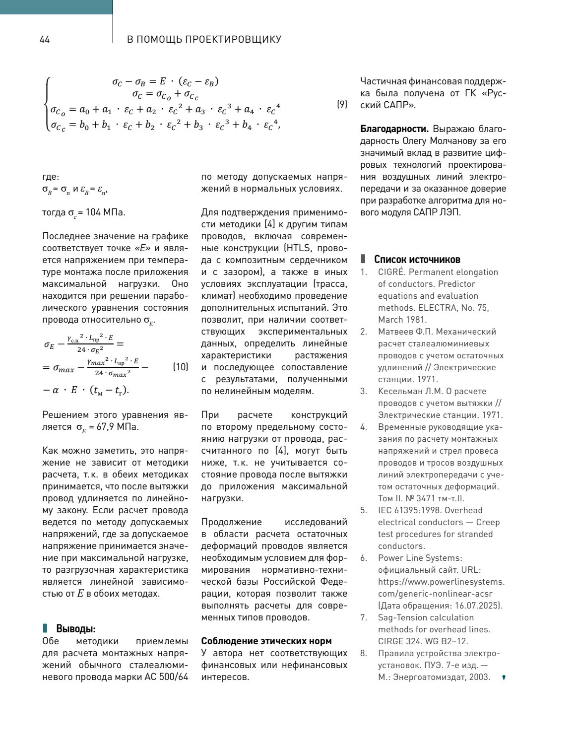
To determine point C, where the linear extension path ends and nonlinear extension resumes, the linear relationship defined by the final modulus of elasticity E is intersected with the nonlinear initial elongation curve:

\left\{ \begin{array}{l} \sigma_C - \sigma_B = E(\varepsilon_C - \varepsilon_B) \\ \sigma_C = \sigma_{C,o} + \sigma_{C,c} \\ \sigma_{C,o} = a_0 + a_1\varepsilon_C + a_2\varepsilon_C^{2} + a_3\varepsilon_C^{3} + a_4\varepsilon_C^{4} \\ \sigma_{C,c} = b_0 + b_1\varepsilon_C + b_2\varepsilon_C^{2} + b_3\varepsilon_C^{3} + b_4\varepsilon_C^{4} \end{array} \right. \tag{9}

Using \(\sigma_B = \sigma_p\) and \(\varepsilon_B = \varepsilon_p\) gives \(\sigma_C = 104\ \mathrm{MPa}\).

The final value on the diagram corresponds to point E: the conductor stress at stringing temperature in the after Max Load condition. It is found by solving the parabolic conductor state equation for \(\sigma_E\):

\sigma_E - \frac{\gamma_{SW}^{2} L_{eq}^{2} E}{24\sigma_E^{2}} = \sigma_{max} - \frac{\gamma_{max}^{2} L_{eq}^{2} E}{24\sigma_{max}^{2}} - \alpha E(t_m - t_g) \tag{10}

The solution is \(\sigma_E = 67.9\ \mathrm{MPa}\). This stress does not depend on the calculation method because both methods assume linear behaviour after permanent elongation. Under the allowable-stress design approach, where the allowable stress is defined by the maximum-load condition, the unloading characteristic is a linear function of E in both methods.

9. Conclusions

Both methods are acceptable for calculating the stringing stresses of a conventional ACSR 500/64 conductor using the allowable-stress method under normal conditions.
To confirm the applicability of method [4] to other conductor types - including modern HTLS conductors, composite-core conductors and gap-type conductors - and to other operating environments, routes and climates, additional testing is required. Where appropriate experimental data are available, this would allow linear elongation characteristics to be established and then compared with nonlinear-model results.
For structural calculations at the second limit state, conductor loads calculated under [4] may be lower because the method does not account for the conductor state after permanent elongation caused by application of the maximum load.
Continued research into permanent conductor deformation is necessary for development of a regulatory and technical framework capable of supporting modern conductor types.

Ethical Compliance and Acknowledgements

The author has no relevant financial or non-financial interests. Partial financial support was provided by Russian CAD Group.

Acknowledgements. The author expresses gratitude to Oleg Molchanov for his significant contribution to the development of digital technologies for overhead transmission line design and for the trust placed in the author during development of an algorithm for a new module of the overhead line CAD software.

References

CIGRE. Permanent elongation of conductors. Predictor equations and evaluation methods. ELECTRA, No. 75, March 1981.
Matveev F. P. Mechanical calculation of steel-aluminium conductors taking permanent elongation into account. Elektricheskie Stantsii, 1971.
Keselman L. M. On conductor calculation taking elongation into account. Elektricheskie Stantsii, 1971.
Temporary Guidelines for Calculation of Stringing Stresses and Sags of Conductors and Earth Wires of Overhead Transmission Lines Taking Permanent Deformation into Account. Volume II. No. 3471 tm-t.II.
IEC 61395:1998. Overhead electrical conductors - Creep test procedures for stranded conductors.
Power Line Systems. Generic Nonlinear ACSR data. Official website. Accessed 16 July 2025.
Sag-Tension Calculation Methods for Overhead Lines. CIGRE 324, WG B2-12.
Rules for Electrical Installations (PUE), 7th ed. Moscow: Energoatomizdat, 2003.

Published Russian original

RUM, No. 2 (624), 2026

The Russian original is shown below as journal pages 38-44, corresponding to PDF pages 39-45.